


 En
En

Magnetic Linear Encoders 101

Magnetic Linear Encoders 101
Introduction
Across modern automation, motion platforms once steered by simple optical transducers now face harsher shop-floor realities: airborne coolant, grinding dust, welding spatter, extreme temperature swings, and electromagnetic interference (EMI) from ever-denser servo drives. In this environment a magnetic linear encoder offers a compelling alternative.
Where an optical glass scale might cloud over or miscount after a single droplet, a linear magnetic encoder happily carries on, its poles hidden beneath a stainless tape and its Hall-effect sensors immune to stray particles. Yet misunderstandings linger: Is the resolution coarse? How does a magnetic encoder linear actually interpret pole transitions? What accuracy is possible with interpolation? How reliable is a linear magnetic encoder strip after years of thermal cycling?
This article answers those questions in one place—spanning fundamentals to integration tips—so that designers, maintenance engineers, and technically curious buyers can specify, install, and troubleshoot with confidence. By the end you will grasp:
The magnetic linear encoder working principle—from pole pitch through sine/cosine generation to digital interpolation.
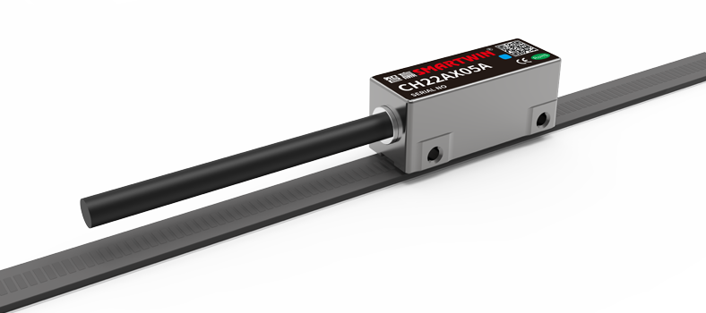
The anatomy of an encoder system: magnetic linear encoder tape (or rigid bar) plus readhead electronics, interface driver, and diagnostic tools.
Signal formats—Incremental 1 Vpp, quadrature A/B/Z, BiSS-C, SSI, PWM—and when each excels.
Calibration, error budgeting, and noise mitigation for micrometer-class accuracy.
While the discussion centers on single-axis position feedback, many principles translate to multi-turn rotary encoders, ring encoders for spindle speed, and hybrid optical-magnetic architectures now emerging in the silicon-photonics era.
A Quick Historical Detour
Early linear encoders were purely mechanical: rack-and-pinion setups delivering step counts to punch cards. Then came 1970s optical scales—chrome graduations on glass read by photodiodes—propelling CNC lathes and coordinate-measuring machines (CMMs) into the sub-micron realm. Optical dominance lasted three decades, but cost, fragility, and cleanliness demands limited broader adoption.
Magnetic alternatives matured quietly in the background. Ferrite tracks on steel carriers could encode a 1 mm pole pitch, but Hall elements had sub-optimal noise and resolution. Everything changed when anisotropic magnetoresistive (AMR) sensors arrived, quickly followed by giant (GMR) and tunneling magnetoresistive (TMR) technology. Resolution below 0.1 µm on a 1 mm pitch suddenly became routine, meeting servo bandwidths once thought exclusive to glass.
Simultaneously, flexible stainless magnetic linear encoder tape—less than 0.3 mm thick, adhesive-backed, cut-to-length—simplified retrofits. Today, from long-travel plasma gantries to compact cobot joints, the magnetic encoder linear is a workhorse, complemented by software interpolation, CRC-checked serial links, and self-diagnostic ASICs.
Magnetic Linear Encoder Working Principle
Pole Generation
Every linear magnetic encoder strip carries alternating north (N) and south (S) poles magnetized at a constant pitch (τ). Common pitches are 1.00 mm, 2.00 mm, and 5.00 mm; shorter pitches yield higher native counts per millimeter but require tighter sensor-to-scale gaps. Magnetization uses a fixture that pulses several kilo-amps through a pole-piece, impressing a pattern onto ferritic stainless or polymer-bonded tape.
Readhead Sensor Array
Inside the readhead a linear array of Hall, AMR, or TMR elements senses the perpendicular component of the magnetic field, Bz. Two groups of sensors are offset by τ/4, ensuring their outputs—call them Sine and Cosine—are 90° electrical apart. Mathematically:
S=A⋅sin(2πx/τ)C=A⋅cos(2πx/τ)S = A·sin(2πx/τ) C = A·cos(2πx/τ)
where A is field amplitude and x the scale displacement relative to the sensor.
Signal Conditioning
Raw micro-volt-level signals pass through low-noise instrumentation amplifiers, anti-alias filters, and automatic gain control. Modern front-end ASICs integrate these steps while embedding temperature sensors. Calibration tables adjust amplitude and phase imbalance, minimizing harmonic distortion that would otherwise impair interpolation.
Digital Interpolation
The conditioned S and C voltages are digitized (12–16 bit ADC). An angle-tracking loop computes
θ=atan2(S,C)θ = atan2(S, C)
Differentiating successive θ samples yields incremental counts. If an encoder interpolates 4 096 positions per pole pair (called ×4096 factor), a 1 mm pitch provides 0.244 µm resolution. Some designs reach ×65 536, hitting 15 nm—well into nanometer territory once reserved for laser interferometers.
Incremental vs. Absolute Coding
Incremental encoders output quadrature A/B edges; motion controllers count these edges and, upon encountering a reference mark Z, zero the position counter. After power-loss the axis must move until it sees Z again.
Absolute encoders embed a secondary track—a pseudorandom or Gray-coded pole sequence. Power-on decoding gives the exact scale position without motion, ideal for vertical axes or medical tables where re-homing is unsafe.
Interface Drivers
RS-422 differential line drivers buffer incremental edges over 10 m cables with minimal skew. Absolute data may use SSI (up to 5 MHz clock) or BiSS-C (32 MHz). Both append cyclic redundancy check (CRC) bits to guarantee data integrity—vital in high-g cobots or EMI-filled weld zones.
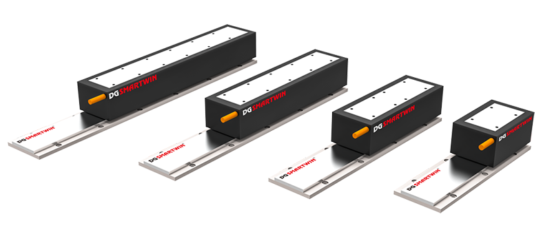
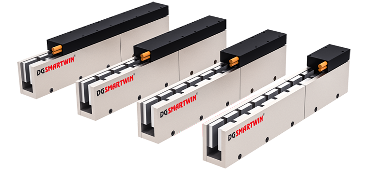
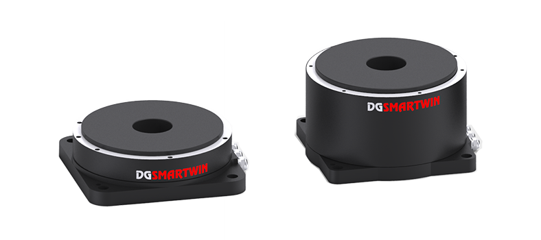
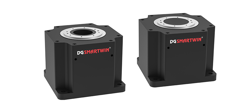
Anatomy of a Magnetic Encoder System
| Sub-assembly | Principal Functions | Typical Materials & Notes |
|---|---|---|
| Magnetic linear encoder strip / tape | Stores pole pattern; provides mechanical datum | Austenitic stainless (non-magnetic substrate) or flexible polymer with embedded ferrite powder; adhesive-back or carrier rail; protective lamination optional. |
| Readhead housing | Shields electronics; maintains sensor gap | CNC-machined aluminum with O-rings and labyrinth seals; LED alignment window; M3 or M4 mounting holes with ±1 mm adjustment slots. |
| Sensor PCB | Hosts Hall/AMR array, ADC, interpolation ASIC | FR-4 or high-temp polyimide if solder reflow > 260 °C; board shielded by Mu-metal if stray fields exceed 5 mT. |
| Cable & Connector | Carry power (5 V/24 V) and signals | PUR-jacketed flex cable, 360° shield crimp, M12 A-coded connector; twisted pairs for A/B/Z. |
| Diagnostic software | Displays amplitude, offset, signal-to-noise, CRC errors | USB dongle or EtherCAT bridge; histogram view to spot stuck bits. |
Mounting gap: Most datasheets specify 0.3 mm – 1.5 mm between tape and sensor. Wider gaps increase immunity to mechanical flutter but reduce field amplitude; designers must verify signal margin at both cold-start and 100 °C running temperatures.
Thermal coefficient: Steel tapes expand ~ 11 ppm/°C, aluminum machine beds ~ 23 ppm/°C. Over a 1.5 m travel, a 20 °C swing can introduce 0.36 mm error if the tape is bonded to aluminum without a differential-CTE compensation algorithm. Premium vendors offer Invar carrier rails (1 ppm/°C) or software linearization tables to mitigate this.
Signal Formats in Depth
Analog 1 Vpp (differential)
Legacy interface still favored in metrology. Two 180°-opposed sine waves centered at 1 V with 0.5 V amplitude. External interpolators can push resolutions beyond ×262 144. Cable length up to 150 m with 120 Ω termination.Incremental A/B/Z (RS-422)
Edge-encoded quadrature: each cycle yields four counts (00 → 01 → 11 → 10). A Z-channel marks every 1 000 poles or custom index. Standard in CNC controllers and many PLCs. At 4 096× interpolation, a 1 m/s move equals 4 MHz edge rate—within reach of modern FPGA counters.PWM
Single-wire (plus ground) position code encoded as duty cycle of a 100 µs frame. Cheap for low-pin microcontrollers in AGV or consumer axes, but jitter (±1 µs) limits sub-micron accuracy.SSI(Synchronous Serial Interface)
Clock-driven readout: master pulses 25–32 bits at 2–5 MHz. Absolute position word plus error flags; supports daisy chain of two encoders. Deterministic latency, making it popular in hydraulic servo valves.BiSS-C / CB / CSI-22
Open-source descendant of SSI; clock up to 32 MHz, CRC-5 or CRC-6 safeguarding. BiSS-Safety variant fits SIL-3 requirements in collaborative robots. Real-time FPGAs can close 4 kHz loops with < 7 µs total delay.**HIPERFACE DSL / EnDat 3 ** (hybrid)
Though more common in rotary motors, linear readheads increasingly embed DSL or EnDat packets on a single-pair along with motor phase power, reducing cable count in battery-electric vehicles.
Accuracy & Error Budget
Total system error (Ex) combines several contributors:
Ex=√(Ep2+Eg2+Einl2+Etc2+Eint2)Ex = √(Ep² + Eg² + Einl² + Etc² + Eint²)
| Symbol | Source | Typical Value |
|---|---|---|
| Ep | Pole-pitch manufacturing tolerance | ±2 µm/m (standard tape) |
| Eg | Scale/readhead gap variation | ±1 µm per 0.1 mm gap change |
| Einl | Interpolation non-linearity (INL) | ±40 nm (×4 096 interpolator) |
| Etc | Thermal coefficient mismatch | 0 – 360 µm over 1.5 m, 20 °C |
| Eint | Controller edge-count jitter & latency | ±0.5 count (quadrature) |
Mitigation strategies:
Install tape on the same material as the moving axis (steel-on-steel).
Use absolute serial data so controller latency does not translate into position lag.
Enable “dynamic amplitude control” in the ASIC to maintain full sine swing as temperature changes.
For ultra-long axes (> 25 m), splice tapes with laser-cut joints and map residual error via laser interferometer, storing corrections in drive firmware.
Design-In Guidelines
Mechanical Reference Faces
Machine a 10 mm-wide ground surface along the axis; mount the magnetic linear encoder strip with a precision-machined aluminum carrier to protect edges from forklifts.Adhesive Selection
For tapes under coolant, choose a 3M™ VHB acrylic foam adhesive rated –40 °C to 150 °C. Use primer on porous cast-iron beds. Clamp with silicone roller 40 N for uniform bond line.Readhead Alignment
LEDs on the housing flash green when the Sine/Cosine amplitude ratio is within ±10 %. Shim using feeler gauges until steady. Torque M3 screws to 0.8 N·m.Cable Routing
Separate encoder cable trays from motor power by 150 mm. Cross at 90° if unavoidable. Terminate shields 360° at drive cabinet entry.Grounding
Bond machine bed, tape carrier, readhead housing, and cabinet star-point with 16 mm² braid. Avoid daisy-chain grounding that forms loops.Firmware Checks
In BiSS-C systems, poll “Warning Amplitude Low” flag; if set for > 1 s, slow the axis and alert operator before count loss occurs.
Troubleshooting Checklist
| Symptom | Likely Cause | Fix |
|---|---|---|
| Position jumps exactly 1 pole (1 mm) | Missing quadrature edge due to weak signal | Clean tape, reduce gap, verify 120 Ω term. |
| CRC error flag in BiSS | EMI burst or cable exceeds 15 m | Add ferrite core; switch to shielded twisted-pair CAT6a. |
| Sinusoid amplitude imbalance >20 % | Readhead yaw misaligned | Loosen screws, rotate < 2° until green LED. |
| Gradual drift vs. laser reference | Thermal mismatch | Switch to Invar carrier or apply software comp. |
| Noise ±1 count static | Ground loop | Isolate encoder shield at one end; add common-mode choke. |
Application Case Studies
CNC Gantry Router (3 × 2 m Travel)
A woodworking OEM replaced 5 µm optical scales (glass) with a 1 mm-pitch magnetic linear encoder tape and ×5 120 interpolating readhead (0.195 µm resolution). Dust tolerance eliminated weekly clean-wipe downtime. Combined with drive jerk limitation, positional repeatability improved from ±8 µm to ±4 µm over 40 °C ambient span.
Collaborative Robot Arm
Each elbow joint needed absolute feedback < 0.02° and SIL-2 functional safety. Engineers embedded 50 mm linear magnetic encoder stripscurved into arcs, read by miniature BiSS-Safety readheads. Start-up position was available in 5 ms, enabling power-on-to-motion under 2 s.
Lithium-Battery Tab-Former
Roll-to-roll forklifts create iron filings; optical strips lasted hours. Switching to nickel-capped magnetic scales plus Hall readheads allowed 24-month MTBF. The system used SSI at 4 MHz; edge-triggered form-die engaged at ±3 µm accuracy.
MRI Patient Table
Conventional encoders malfunction inside 1.5 T MRI bore. A non-ferrous linear magnetic encoder strip bonded to carbon-fiber, read by TMR sensors with zero ferromagnetic material, delivered 0.5 mm accuracy over 2 m. PWM output (plastic-optical-fiber isolated) avoided ground loops.
Future Trends
TMR & GMR Miniaturization: 3 µm sensor pitch allows ≥ 10 000× interpolation on 0.5 mm pole tape—opening nanoscale metrology for semiconductor steppers.
Hybrid Optical-Magnetic: Dual tracks—optical for nanometer resolution, magnetic for homing redundancy—enter aerospace actuators requiring triple-redundant feedback.
Embedded Machine Learning: On-board Cortex-M cores train anomaly-detection models; readheads can flag “bearing wear” when vibration signature modulates sine amplitude.
Silicon-Photonics Encoders: Waveguide interference patterns etched in silicon nitride read Hall-based pole sequences—combining photonics resilience with magnetic absolute coding.
Wireless Power & Data: For linear motors in sealed pharma isolators, energy harvesting coils inside readhead power BLE transmitters; 12 kbps absolute position travels over 5 cm airgap, replacing slip-torsion cables.
Summary & Key Takeaways
A magnetic linear encoder marries a pole-patterned linear magnetic encoder strip with a Hall/AMR/TMR readhead to generate sine/cosine voltages. Interpolating ASICs subdivide each pole pitch into thousands of digital counts. Output may be analog (1 Vpp), incremental quadrature (A/B/Z), or absolute serial (SSI, BiSS-C).
The architecture offers:
Contamination immunity—perfect for oil-soaked machine tools.
Wide mounting gaps—simpler mechanical tolerances.
Large temperature range—-40 °C to 125 °C with proper compensation.
Cost-effectiveness—flexible magnetic linear encoder tape installs in minutes.